Feel free to browse through projects via the blue links provided below. Enjoy this digital experience of problem solving and critical thinking.
Part 1:
Go to Project 1 - Data Engineering
Go to Project 2 - Data Science
Go to Project 3 - Analytics and Visual Ouput
Part 2:
Go to Project 4 - Cloud Computing
Go to Project 5 - Unit Testing
Go to Project 6 - CyberSecurity
Go to Project 7 - GDPR Offuscator Draft
Go to Project 8 - Refactoring Machine Learning processes
The projects presented here are all interconnected. The task here is to build an automated data management system that will feed a Deep Learning Neural Network for predictions. Further illustrations will be presented along to provide further references.
You can visit the Git repository for this portfolio website via the following link: Visit the Git repository
In this section an automated ETL (Extract / Transform / Load) pipeline is being setup to handle data from a remote database. The pipeline output is an ingestion data lake connected a local data warehouse where processed data are stored in a STAR schema (relational databases) for further processing in the Data Science project that will follow.
Relational databases can created with PostgreSQL which can be intalled with the following command on Linux:
pip install psql
A virtual environment is then created for testing purposes to ensure that the software is robust and always working. For testing the library Pytest is being used while a MakeFile ensures automation during deployment.
A virtual environment can be created with the following commands:
pip install pyenv
python -m venv venv
Loading the virtual environment:
source venv/bin/activate
Exporting the python path to the environment:
export PYTHONPATH=$PWD
Pytest can be installed in the virtual environment with the following command:
pip install pytest
A requirement file is ideal in this case to store all the list of packages required for the project and to be installed all at once:
pip freeze > requirements.txt
pip install -r requirements.txt
Autopep8 is added to the list for PEP-8 compliance.
Safety and Bandit check for any issues such as SQL injections.
Coverage is a package that checks how much of the code is being tested.
The entire automation procedure is then deployed remotely, essentially by running a Makefile in Bash script.
The example dataset is accessed via the following link:
\link>
\img>
Those data are static for now but ideally the management system should eventually be able to handle new sets of data dynamically using a cloud computing platform such as Amazon Web Services (AWS) and Terraform. You can view a version of a pipeline previously built with AWS and AWS Lambda
The data consist of a training set and a testing set each detailling screen dots with x and y coordinates from handwritten data from a touch-screen device. Validation data are also included in this case which means it is possible to assess whether the model's predictions were true or not.
The bot must accurately ingest the data and carry timestamp processing tasks, then store the procesed data in a data warehouse for the purpose of the Data Science project, all in order to translate the hand written letters.
Pandas libraries provide robust packages that enable processors to handle pkl formats and Json protocols efficiently. The code for ingestion is pretty straightforward and looks as below:
#import Pandas libraries
import pandas as pd
# Loading the training dataset
# An util folder may ideally be created later for reused functions
def load_data():
f = gzip.open('mnist.pkl.gz', 'rb')
f.seek(0)
training_data, validation_data, test_data = pickle.load(f, encoding='latin1')
f.close()
return (training_data, validation_data, test_data)
training_data, validation_data, test_data = load_data()
training_data
# Printing datasets details
print("The feature dataset is:" + str(training_data[0]))
print("The target dataset is:" + str(training_data[1]))
print("The number of examples in the training dataset is:" + str(len(training_data[0])))
print("The number of points in a single input is:" + str(len(training_data[0][1])))
The data warehouse is designed in three stages:
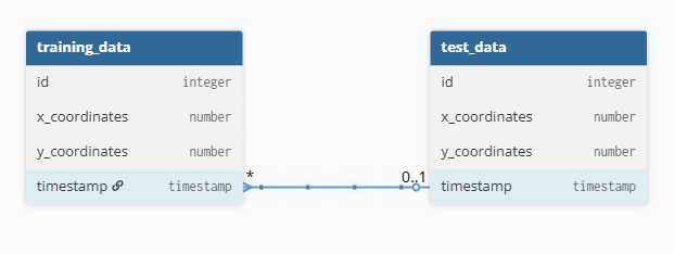
- Concept: Storing loaded training and test datasets in a relational database in a STAR schema. The data warehouse will contain two tables: the training table and the test table.
- Logic: Primary keys and timestamps are assigned to data points from the data sets to allow dynanamic data tracking and time series analysis.
- Physic: PostgreSQL will be used to create the database and relational tables via the python script. The tables will be linked by the timestamps attribute in the Entity Relationship Diagram.
The local database and tables can be created using the Psycopg2 library. A dedicated warehouse_handler.py facilitate debugging while carrying this task.
Let's create our data warehouse with psql using Psycopg2:
import psycopg2 from psycopg2 import sql try: # Connecting to the default 'postgres' database connection = psycopg2.connect( dbname="postgres", user="hgrv", password="hgrv_pass", host="localhost", port="5432" ) connection.autocommit = True # Enable autocommit for database creation # Creating a cursor object for SQL script cursor = connection.cursor() # Checking whether the database already exists cursor.execute( sql.SQL("SELECT 1 FROM pg_database WHERE datname = %s"), [data_warehouse] ) exists = cursor.fetchone() # Creating the table for the first instance if not exists: # Defining a name for the database for the first instance database_name = "data_warehouse" # Executing a SQL command to create the database if it does not already exist (first instance only) cursor.execute(sql.SQL("CREATE DATABASE {}").format(sql.Identifier(database_name))) print(f"Database '{data_warehouse}' created successfully!") else: print(f"Database '{data_warehouse}' already exists.") except Exception as e: print(f"Error: {e}") print(f"Check the debugging console for any error in the SQL script.")
Note: The same result is achievable with Pg8000 (ideal for low-load applications without C-denpendencies). You can check the specific differences between Pg8000 and psycopg2 on the following link: https://www.geeksforgeeks.org/python/difference-between-psycopg2-and-pg8000-in-python/
Let's add the tables that will store the following corresponding attributes: 'id' (primary key), 'x-coordinates' and 'y-coordinates'. The connection and cursor
try: # SQL query to create a table create_table_query = """ CREATE TABLE IF NOT EXISTS test_data ( id SERIAL PRIMARY KEY, x_coordinates NUMERIC(10, 2), y_coordinates NUMERIC(10, 2), timestamp DATE DEFAULT CURRENT_DATE ); CREATE TABLE IF NOT EXISTS training_data ( id SERIAL PRIMARY KEY, x_coordinates NUMERIC(10, 2), y_coordinates NUMERIC(10, 2), timestamp DATE ); """ # Executing the query cursor.execute(create_table_query) connection.commit() # Save changes to the database print("Table 'employees' created successfully!") except Exception as error: print(f"Error occurred: {error}") print(f"Check for any error in the SQL script.")
At this point, the data warehouse can be updated with the current load of data sets:
try: # Data to insert # training_data_to_insert = (train_set_x, train_set_y, timestamp_current) # test_data_to_insert = (test_set_x, test_set_y, timestamp_current) # Inserting x-coordinates, and timestamp into table 'training_data' for item in train_set_x: # Data to insert training_data_to_insert = item # SQL query to insert data into tables insert_query = """ INSERT INTO training_data (x_coordinates, timestamp) VALUES (train_set_x, timestamp_current) """ # Execute the query cursor.execute(insert_query, training_data_to_insert) # Commit the SQL script connection.commit() # Inserting y-coordinates into table 'training_data' for item in train_set_y: # Data to insert training_data_to_insert = item # SQL query to insert data into tables insert_query = """ INSERT INTO training_data (y_coordinates) VALUES (item, timestamp_current) """ # Execute the query cursor.execute(insert_query, training_data_to_insert) # Commit the SQL script connection.commit() # Inserting x-coordinates, and timestamp into table 'test_data' for item in test_set_x: # Data to insert test_data_to_insert = item # SQL query to insert data into tables insert_query = """ INSERT INTO test_data (x_coordinates, timestamp) VALUES (item, timestamp_current) """ # Execute the query cursor.execute(insert_query, test_data_to_insert) # Commit the SQL script connection.commit() # Inserting y-coordinates into table 'test_data' for item in train_set_y: # Data to insert test_data_to_insert = item # SQL query to insert data into tables insert_query = """ INSERT INTO test_data (y_coordinates) VALUES (item, timestamp_current) """ # Execute the query cursor.execute(insert_query, test_data_to_insert) # Commit the SQL script connection.commit() print("Data inserted successfully into {data_warehouse}!") except Exception as error: print(f"Error occurred: {error}") print(f"Check for any error in the SQL script.") finally: # Closing the cursor and connection cursor.close() connection.close() print("PostgreSQL connection is now closed.")
These 'try-except-finally' clauses are then put together in a function update_data_base() invoqued in the neural_layers.py file. We must also ensure that there are no duplicates due to the random pixel effect of handwriting on a touchscreen or touchpad.
In later projects when setting up the enpoint of an API, those SQL commands must always ensure that no injection occurs during queries.
To make the designed platform more interactive, engaging and intersting, an API can be built to request the website user to suggest optimisation parameters before running the projects scripts, for the purpose of the following Data Science project:
import requests def get_suggestion(number): url = "http://numbersapi.com/{}".format(number) r = requests.get(url) if r.status_code == 200: print(r.text) else: print("An error occurred, code={}".format(r.status_code))
The code can be refactored later in the project in order to intercept errors with user friendly messages and hints for conflicts resolution. This API can then be ran in the corresponding app or module as follows:
import api api.get_suggestion(input("Enter a number to suggest layers density (Ex: 35): "))
APIs essentially act as simplified communication bridges between various software components and devices.
The orchestration of dependencies is then updated in the Makefile to reflect requirements changes and refresh the virtual environment for processing purposes, deep learning and automation:
# Define the variables for the Python interpreter VENV = venv PYTHON = $(VENV)/bin/python3 PIP = $(VENV)/bin/pip # Declare phony target with no prerequisites .PHONY: run clean test pythonpath # Creating first rule to run the app in the virtual environment: run: venv/bin/activate $(PYTHON) src/app.py # Run the neural network in the virtual environment with the app as prerequisite run_neural_network: venv/bin/activate, run $(PYTHON) src/neural_layers.py # Creating virtual environment with updated dependencies venv/bin/activate: requirements.txt python3 -m venv venv $(PIP) install -r requirements.txt # Setting the python path to the current working directory pythonpath: venv/bin/activate export PYTHONPATH=$PWD # Run tests test: venv/bin/activate $(PYTHON) -m unittest discover -s tests # Clean up .pyc files and refresh clean: find . -name "*.pyc" -delete rm -rf __pycache__ rm -rf venv
Once all the handling modules have been set, a backend neural network for deep learning can be added at the end of the pipeline to generate relevant visual outputs and predictive metrics.
In this section a Neural Network is being added with optimised hyper-parameters using the Python API of Tensorflow. Tensorflow is a very popular tool used to build and deploy Neural Network. Hence for the purpose of this project, Tensorflow will be the computing framework for batch processing while compiling will be handled by importing the Keras library.
One great advantage of using Tensorflow is that one does not need to write code for the feedforward and back-propagation, but only to set the hyper-parameters such as density of spare weights matrix or the number of neurons and layers as well as the activation function for the last layer.
The chart below illustrates the multilinear neural network for one data point:
Cumulative input = wT*x + b = w1*x1 + w2*x2 + wk*xk + b
The chart below illustrates the batch processing matrix for a given batch size after feedforward and back-propagation for weights calibration:
Chart:
There are generally 6 main steps needed in order to implement a neural network model in Keras:
""" The loading has already been implemented in Project 1 as an ingestion pipeline with Pandas libraries. Let's process the data with a wrapper and one-hot encoding (handling database columns in arrays) and assign the timestamp reference. """ # Importing the Python module Datetime to handle timestamping tasks at the end of each loading phase from datetime import datetime # Setting the one_hot encoding for the target value def one_hot(j): """ - input is the target dataset of shape (1, m) where m is the number of data points - returns a 2 dimensional array of shape (10, m) where each target value is converted to a one hot encoding - Look at the next block of code for a better understanding of one hot encoding """ n = j.shape[0] new_array = np.zeros((10, n)) index = 0 for res in j: new_array[res][index] = 1.0 index = index + 1 return new_array data = np.array([0, 1, 2, 3, 4, 5, 6, 7, 8, 9]) one_hot(data) # Defining the data_wrapper function def data_wrapper(): tr_d, va_d, te_d = load_data() training_inputs = np.array(tr_d[0][:]).T training_results = np.array(tr_d[1][:]) train_set_y = one_hot(training_results) validation_inputs = np.array(va_d[0][:]).T validation_results = np.array(va_d[1][:]) validation_set_y = one_hot(validation_results) test_inputs = np.array(te_d[0][:]).T test_results = np.array(te_d[1][:]) test_set_y = one_hot(test_results) return (training_inputs, train_set_y, validation_inputs, validation_set_y) # Calling the data_wrapper() function and assigning the output to local variables train_set_x, train_set_y, test_set_x, test_set_y = data_wrapper() # Transposing the sets to ensure that the data-Matrix is in the correct shape train_set_x = train_set_x.T train_set_y = train_set_y.T test_set_x = test_set_x.T test_set_y = test_set_y.T # Checking that the sets are in the desired shape print ("train_set_x shape: " + str(train_set_x.shape)) print ("train_set_y shape: " + str(train_set_y.shape)) print ("test_set_x shape: " + str(test_set_x.shape)) print ("test_set_y shape: " + str(test_set_y.shape)) # Getting current timestamp timestamp_current = datetime.now().strftime("%d%m%Y %H%M%S") print('Latest database timestamp: {timestamp_current}') """ Timestamps details: %d: Day of the month (01-31). %m: Month (01-12). %Y: Year in four digits. %H: Hour in 24-hour format (00-23). %M: Minutes (00-59). %S: Seconds (00-59). """
Notice that before batch processing, data are usually pre-processed or cleaned beforehand to fit the dimensions of a processing matrix (In this case dimension (n, m) for n data points and m layers for the overall feedforward and back-propagation)
It is also common practice to timestamp the data to ensure data integrity and generate timeseries for analysis, for instance in cases where seasonality would seem to be a strong empiric factor on the predictions.
# Creating first instance of sequential neural model and adding density (layers, activation function, regulariser) # First instance without layers nn_model = Sequential() # Adding a Dropout for the first layer at 0.3% of neurons in Bayesian dropout for each iteration in order to generate a sparse weight matrix after cumulative input nn_model.add(Dropout(0.3)) # Initialising first hidden layer with 35 neurons, 28x28 = 784 components in the input vectors and 'relu' activation function # nn_model.add(Dense(35, input_dim=784, activation='relu')) # refactored to request density level from user nn_model.add(Dense(density_level, input_dim=784, activation='relu')) # Regularising the interconnected neural network nn_model.add(Dense(21, activation = 'relu', kernel_regularizer = regularizers.l2(0.01))) # Setting a last softmax layer with 10 classes nn_model.add(Dense(10, activation='softmax'))
# Compiling and optimising the predictive model with the crossentropic loss function nn_model.compile(loss='categorical_crossentropy', optimizer='adam', metrics=['accuracy'])
# Fitting the model with a minibatch of size 10 and 10 epochs nn_model.fit(train_set_x, train_set_y, epochs=10, batch_size=10)
# Evaluating the model's scores and printing the accuracy in the training dataset scores_train = nn_model.evaluate(train_set_x, train_set_y) print("\n%s: %.2f%%" % (nn_model.metrics_names[1], scores_train[1]*100))
# Setting the predictions on the test dataset predictions = nn_model.predict(test_set_x) predictions = np.argmax(predictions, axis = 1) predictions
Note the great advantage of Keras' default use of Tensorfow as backend ("backend":"tensorflow") in the 'keras.json' file.
Note also that batch normalisation in Keras libraries makes efficient use of empirically proven methods too: Here for instance, a specific minimal constant (epsilon) is being added to the Variance to ensure that the standard deviation is never nil during normalisation. Batch normalisation in Keras is being implemented with the following code where the 'axis= -1' specifies a normalisation across rows:
nn_model.add(BatchNormalization(axis=-1, epsilon=0.001, beta_initializer='zeros', gamma_initializer='ones'))
In this section new data stored in the data warehouse are used to train the neural network continually and produce a visual chart for further monitoring of the data and the model's apparent behaviour.
In Keras, the imported Numpy and Matplotlib modules are working dynamically using the Tensorflow backend. A visual outut of the data may be implemented with Keras as follows:
# Visualising the dataset by index to check correct labelling index = 1000 k = train_set_x[index,:] k = k.reshape((28, 28)) plt.title('Label is {label}'.format(label= training_data[1][index])) plt.imshow(k, cmap='gray') # Visualising different test cases for assessment against validation data index = 9997 k = test_set_x[index, :] k = k.reshape((28, 28)) plt.title('Label is {label}'.format(label=(predictions[index], np.argmax(test_set_y, axis = 1)[index]))) plt.imshow(k, cmap='gray')
The model is eventually being assessed in this data lake to determine its current accuracy metrics for the training dataset and the test dataset:
# Evaluating the model's scores and printing the accuracy in the training dataset scores_train = nn_model.evaluate(train_set_x, train_set_y) print("\n%s: %.2f%%" % (nn_model.metrics_names[1], scores_train[1]*100)) # Setting the predictions on the test dataset predictions = nn_model.predict(test_set_x) predictions = np.argmax(predictions, axis = 1) predictions # Setting scores and printing the accuracy in the test dataset scores_test = nn_model.evaluate(test_set_x, test_set_y) print("\n%s: %.2f%%" % (nn_model.metrics_names[1], scores_test[1]*100))
Relevant local variables and interactive data can also be visualised dynamically with the use of JavaScript to display variables from the Python environment. In terms of added functionalities however, other Software Engineering frameworks, such as React (JavaScript librairy) or node.js (JavaScript runtime environment) for example, can also provide highly efficient ways to build similar frontend projects.
In this regard, it is worth noting the power of Python 3 and JavaScript alone during automation and interactive displays as JavaScript can also effectively be used to run the backend python file, while handling frontend tasks with high efficiency.
In order to illustrate this concept, a request from is added to the html file for this present wepage, and displayed as below prompting the user to suggest a density level between 10 and 100 with or a default value of 35:
<form action="/process.php method="POST" class="" ">
<label for="density" class="">
<p class="">
Enter a density level for your
installed neural network:
</p>
</label><br>
<input class="" type="text" id="density" name="density" value="35"><br>
<input class="" type="submit" value="Submit" disabled>
</form>
Here below is the result after adding that script to the html file for this present webpage at the desired display point:
Notice however that classes are also added later to hml elements to enable control of size, police, colours and display from the CSS script (Updated code in the repository). Let's deploy our designed frontend point:
(Above: Simulation of a display point on the user interface with input-box enabled and 'Submit' button currently disabled.)
Now our frontend point is almost good to go (with the 'Submit' button still desactivated), and a PHP file can specify the actions for the target buttons on the server side (Note that this can also be achieved effectively with Node.js, Python Flask, Django, React or Javascript which are all flexible options; PHP is somehow useful as it precedes and overtakes Html protocols for faster displays).
Html actions can be set by updating the form parameters with ' action="process.php" method="post" ', while using javascript to specify the action in the process.php file:
<?php // Using a JavaScript if-statement to trigger the action if ($_SERVER['REQUEST_METHOD'] === 'POST' && isset($_POST['form'])) { // logic of the action after the setting has been submitted by the user echo "Density level submitted successfully! JavaScript executed via PHP script."; echo "Get set and ready for the next phase of this presention!"; } ? >
This process is using JavaScript to trigger the action written in the PHP file. For this purpose, the setting ' onclick="callPHP()" ' is added as a property of the button element, and the html file can be updated with the following javascript:
<script> function callPHP() { fetch('process.php', { method: 'POST' }) .then(response => response.text()) .then(data => alert(data)); } </script>
Let's deploy our resulting user interface on the display point below (with the 'Submit' button enabled this time!) and also update the last pipelines connections to test that the actions are being triggered on submission:
('Submit' button enabled after implementing last connections for testing and debugging purposes.)
Keeping in mind that the variable density_level was set when buiding the API, a visual rendering can be designed from the front end. Python makes this possible by implementing an update_density module in the API as you can see in the commented code below:
from flask import Flask, request app = Flask(__name__) # Decorating a submit_density() function with the form's action and method @app.route('/submit', methods=['POST']) def update_density(): density = request.form['density'] # Accessing form density from user input return density # Enabling detailed error tracebacks during development on main module. if __name__ == '__main__': app.run(debug=True)
(The simple Flask App script above creates an updating unit module ready for import within the API.)
For presentation purposes, let's use Data Engineering skills to also deploy a 'Start' button using the Javascript fecth() module to interact indirectly with the Make's API via a webhook in order to promt the website user to start a demonstration of the project in trial version. The Make's API allows to trigger workflows in JavaScript by using automated HTTP requests:
< class="greybox"># The webhook url is set up in Make by creating an account and creating a scenario # that is triggered in Javascript as below: const triggerWebhook = async () => { const response = await fetch('https://hook.make.com/PROJECTS_WEBHOOK_URL', { method: 'POST', headers: { 'Content-Type': 'application/json' }, body: JSON.stringify({ key: 'value' }), }); if (response.ok) { console.log('Webhook triggered successfully!'); } else { console.error('Failed to trigger webhook:', await response.text()); } }; triggerWebhook();
Note that The same result is also achievable with Node.js which is also a very popular option for frontend application and software development projects. Typically in such Python Web environments data are commonly extracted from parsed data handled by servers with POST and Get Requests.
Let's deploy the 'Start' button:
You can try to visualise the output of the whole pipeline yourself with our last settings-box deployed above by clicking the 'Submit' button, which will also trigger the Makefile as well as related backend modules in the virtual python environment. Once the project is fully installed, visual outputs of data should be generated on the frontend user interface by Matplotlib using the Tensorflow framework in Keras.
You should however note that our Javascript handlers are also embedded within the html file to ensure that the modules will still be ran in browsers unable to handle PHP requests from the server side.
We must also update our Javascript to trigger the update_density() function from our Flask App, so that the 'Start' button can be ready to run the updated neural network.
- To be updated -
Terraform scripts
Serverless applications with AWS Lambda
Scalabilty and tags for higher efficiency
Testing with Pytest and Moto
PEP8 testing modules
- To be updated -
Under UK domestic law, the General Data Protection Regulation or UK GDPR is a comprehensive data protection law that came into effect on 25 May 2018, alongside an revised version of the Data Protection Act 2018.
According to www.gov.uk/data-protection, data protection in the UK is mainly governed by the UK GDPR and the Data Protection Act of 2018. UK data protection principles specifically restricts how personal information is used by organizations in order to ensure data protection and privacy for individuals (data subjects).
These ‘data protection principles’ are strict rules requiring that people or entities responsible for using personal data must ensure (unless an exemption applies) the following legal requirements are met:
- Fair, lawful and transparent use of data
- Use of information for specific purposes
- Adequate and relevant use of information limited to only necessary data
- Accuracy and update of information
- Data Storage no longer than is necessary
- Appropriate data integrity and security, including protection against unlawful or unauthorised processing, access, loss, destruction or damage
In addition to those legal requirements, there is also a strong emphasis on the processing of more sensitive data (Ex: race, ethnicity, religion, biometric id, health, background checks etc.) as data subjects carry fundamental rights such as the right to transparency and access to information, right to rectification/erasure, objections and also restrictions on automated decision-making. Therefore personal data must also be handled in accordance with these principles.
The GDPR framework described previously actually constitutes the rationale for building and Obfuscator to secure sensitive data. In this project we will precisely follow those personal data guidelines as stated in the UK legislation at:
https://www.legislation.gov.uk/eur/2016/679/contentsThe Principles relating to processing of personal data (Article 5 to Article 11A)
Building our Data Obfuscator under GDRP regulation and guidelines ensures that data processing platforms can have a viable option at hand providing up to date and secured solutions.
Building a fully tested and automated GDPR Obfuscator for deployment on AWS and third-party software integration.
Linux CLI
Python 3
Terraform
Pytest
Boto3
Moto
Make
- System Requirements
- Installation
- AWS Deployment
- Integration
- Note on Terraform deployment and Passkeys
- Note on Unit-Testing and Mock-Tests
- Obfuscation principles
- Moto, Boto3
- Terraform documentation
- Amazon Web Services (AWS)
All commercial rights related to this project are reserved by the owner TechReturners (Copyright 2025).
- To be updated soon -
Empirically proven methods for hyper-parameters optimisation and initialisation
Visualising Neural Networks with JavaScript librairies and Node.js